
VLOOKUP has limitations…
When you have a piece of information you know and want to lookup something else in a column to its right in a large data table, VLOOKUP has always been the “go to” function to use!
But there are problems with VLOOKUP…
- The data you want to lookup has to be to the RIGHT of the data you know
- VLOOKUP can’t return multiple columns of data in one go
Luckily, with the advent of the 365 version of Excel, Microsoft have added a new function that solves these problems, it’s called XLOOKUP.
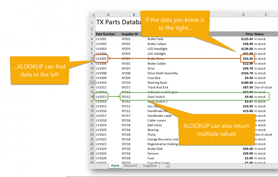
So now you can use XLOOKUP to return values to the left of the “value you know” and a series of values all at the same time as well.
=XLOOKUP(lookup value, lookup array, return array, if not found, match mode, search mode)
It does this by now having two ranges that are selected (to VLOOKUP’s one), lookup array is the range is the area your “value you know” is located, while return array is the area that the result will come from, (no need to count across columns as you did with VLOOKUP).
It also includes a useful option to specify what should be returned if no match is found and also the ability to define the type of match and how XLOOKUP searches through the data.
To see how an XLOOKUP is used, watch the following short video demo…